In last week’s blog post, we discussed gradient descent, a first-order optimization algorithm that can be used to learn a set of classifier coefficients for parameterized learning.
However, the “vanilla” implementation of gradient descent can be prohibitively slow to run on large datasets — in fact, it can even be considered computationally wasteful.
Instead, we should apply Stochastic Gradient Descent (SGD), a simple modification to the standard gradient descent algorithm that computes the gradient and updates our weight matrix W on small batches of training data, rather than the entire training set itself.
While this leads to “noiser” weight updates, it also allows us to take more steps along the gradient (1 step for each batch versus 1 step per epoch), ultimately leading to faster convergence and no negative affects to loss and classification accuracy.
To learn more about Stochastic Gradient Descent, keep reading.
Looking for the source code to this post?
Jump right to the downloads section.
Stochastic Gradient Descent (SGD) with Python
Taking a look at last week’s blog post, it should be (at least somewhat) obvious that the gradient descent algorithm will run very slowly on large datasets. The reason for this “slowness” is because each iteration of gradient descent requires that we compute a prediction for each training point in our training data.
For image datasets such as ImageNet where we have over 1.2 million training images, this computation can take a long time.
It also turns out that computing predictions for every training data point before taking a step and updating our weight matrix W is computationally wasteful (and doesn’t help us in the long run).
Instead, what we should do is batch our updates.
Updating our gradient descent optimization algorithm
Before I discuss Stochastic Gradient Descent in more detail, let’s first look at the original gradient descent pseudocode and then the updated, SGD pseudocode, both inspired by the CS231n course slides.
Below follows the pseudocode for vanilla gradient descent:
while True:
	Wgradient = evaluate_gradient(loss, data, W)
	W += -alpha * Wgradient
And here we can see the pseudocode for Stochastic Gradient Descent:
while True:
	batch = next_training_batch(data, 256)
	Wgradient = evaluate_gradient(loss, batch, W)
	W += -alpha * Wgradient
As you can see, the implementations are quite similar.
The only difference between vanilla gradient descent and Stochastic Gradient Descent is the addition of the
next_training_batchfunction. Instead of computing our gradient over the entire
dataset, we instead sample our data, yielding a
batch.
We then evaluate the gradient on this
batchand update our weight matrix W.
Note: For an implementation perspective, we also randomize our training samples before applying SGD.
Batching gradient descent for machine learning
After looking at the pseudocode for SGD, you’ll immediately notice an introduction of a new parameter: the batch size.
In a “purist” implementation of SGD, your mini-batch size would be set to 1. However, we often uses mini-batches that are > 1. Typical values include 32, 64, 128, and 256.
So, why are these common mini-batch size values?
To start, using batches > 1 helps reduce variance in the parameter update, ultimately leading to a more stable convergence.
Secondly, optimized matrix operation libraries are often more efficient when the input matrix size is a power of 2.
In general, the mini-batch size is not a hyperparameter that you should worry much about. You basically determine how many training examples will fit on your GPU/main memory and then use the nearest power of 2 as the batch size.
Implementing Stochastic Gradient Descent (SGD) with Python
We are now ready to update our code from last week’s blog post on vanilla gradient descent. Since I have already reviewed this code in detail earlier, I’ll defer an exhaustive, thorough review of each line of code to last week’s post.
That said, I will still be pointing out the salient, important lines of code in this example.
To get started, open up a new file, name it
sgd.py, and insert the following code:
# import the necessary packages
import matplotlib.pyplot as plt
from sklearn.datasets.samples_generator import make_blobs
import numpy as np
import argparse

def sigmoid_activation(x):
	# compute and return the sigmoid activation value for a
	# given input value
	return 1.0 / (1 + np.exp(-x))

def next_batch(X, y, batchSize):
	# loop over our dataset `X` in mini-batches of size `batchSize`
	for i in np.arange(0, X.shape[0], batchSize):
		# yield a tuple of the current batched data and labels
		yield (X[i:i + batchSize], y[i:i + batchSize])
Lines 2-5 start by importing our required Python packages. Then, Line 7 defines our
sigmoid_activationfunction used during the training process.
In order to apply Stochastic Gradient Descent, we need a function that yields mini-batches of training data — and that is exactly what the
next_batchfunction on Lines 12-16 does.
The
next_batchmethod requires three parameters:
X
: Our training dataset of feature vectors.y
: The class labels associated with each of the training data points.batchSize
: The size of each mini-batch that will be returned.
Lines 14-16 then loop over our training examples, yielding subsets of both
Xand
yas mini-batches.
Next, let’s parse our command line arguments:
# import the necessary packages
import matplotlib.pyplot as plt
from sklearn.datasets.samples_generator import make_blobs
import numpy as np
import argparse

def sigmoid_activation(x):
	# compute and return the sigmoid activation value for a
	# given input value
	return 1.0 / (1 + np.exp(-x))

def next_batch(X, y, batchSize):
	# loop over our dataset `X` in mini-batches of size `batchSize`
	for i in np.arange(0, X.shape[0], batchSize):
		# yield a tuple of the current batched data and labels
		yield (X[i:i + batchSize], y[i:i + batchSize])

# construct the argument parse and parse the arguments
ap = argparse.ArgumentParser()
ap.add_argument("-e", "--epochs", type=float, default=100,
	help="# of epochs")
ap.add_argument("-a", "--alpha", type=float, default=0.01,
	help="learning rate")
ap.add_argument("-b", "--batch-size", type=int, default=32,
	help="size of SGD mini-batches")
args = vars(ap.parse_args())
Lines 19-26 parse our (optional) command line arguments.
The
--epochsswitch controls the number of epochs, or rather, the number of times the training process “sees” each individual training example.
The
--alphavalue controls our learning rate in the gradient descent algorithm.
And finally, the
--batch-sizeindicates the size of each of our mini-batches. We’ll default this value to be 32.
In order to apply Stochastic Gradient Descent, we need a dataset. Below we generate some data to work with:
# import the necessary packages
import matplotlib.pyplot as plt
from sklearn.datasets.samples_generator import make_blobs
import numpy as np
import argparse

def sigmoid_activation(x):
	# compute and return the sigmoid activation value for a
	# given input value
	return 1.0 / (1 + np.exp(-x))

def next_batch(X, y, batchSize):
	# loop over our dataset `X` in mini-batches of size `batchSize`
	for i in np.arange(0, X.shape[0], batchSize):
		# yield a tuple of the current batched data and labels
		yield (X[i:i + batchSize], y[i:i + batchSize])

# construct the argument parse and parse the arguments
ap = argparse.ArgumentParser()
ap.add_argument("-e", "--epochs", type=float, default=100,
	help="# of epochs")
ap.add_argument("-a", "--alpha", type=float, default=0.01,
	help="learning rate")
ap.add_argument("-b", "--batch-size", type=int, default=32,
	help="size of SGD mini-batches")
args = vars(ap.parse_args())

# generate a 2-class classification problem with 400 data points,
# where each data point is a 2D feature vector
(X, y) = make_blobs(n_samples=400, n_features=2, centers=2,
	cluster_std=2.5, random_state=95)
Above we generate a 2-class classification problem. We have a total of 400 data points, each of which are 2D. 200 data points belong to class 0 and the remaining 200 to class 1.
Our goal is to correctly classify each of these 400 data points into their respective classes.
Now let’s perform some initializations:
# import the necessary packages
import matplotlib.pyplot as plt
from sklearn.datasets.samples_generator import make_blobs
import numpy as np
import argparse

def sigmoid_activation(x):
	# compute and return the sigmoid activation value for a
	# given input value
	return 1.0 / (1 + np.exp(-x))

def next_batch(X, y, batchSize):
	# loop over our dataset `X` in mini-batches of size `batchSize`
	for i in np.arange(0, X.shape[0], batchSize):
		# yield a tuple of the current batched data and labels
		yield (X[i:i + batchSize], y[i:i + batchSize])

# construct the argument parse and parse the arguments
ap = argparse.ArgumentParser()
ap.add_argument("-e", "--epochs", type=float, default=100,
	help="# of epochs")
ap.add_argument("-a", "--alpha", type=float, default=0.01,
	help="learning rate")
ap.add_argument("-b", "--batch-size", type=int, default=32,
	help="size of SGD mini-batches")
args = vars(ap.parse_args())

# generate a 2-class classification problem with 400 data points,
# where each data point is a 2D feature vector
(X, y) = make_blobs(n_samples=400, n_features=2, centers=2,
	cluster_std=2.5, random_state=95)

# insert a column of 1's as the first entry in the feature
# vector -- this is a little trick that allows us to treat
# the bias as a trainable parameter *within* the weight matrix
# rather than an entirely separate variable
X = np.c_[np.ones((X.shape[0])), X]

# initialize our weight matrix such it has the same number of
# columns as our input features
print("[INFO] starting training...")
W = np.random.uniform(size=(X.shape[1],))

# initialize a list to store the loss value for each epoch
lossHistory = []
For a more through review of this section, please see last week’s tutorial.
Below follows our actual Stochastic Gradient Descent (SGD) implementation:
# import the necessary packages
import matplotlib.pyplot as plt
from sklearn.datasets.samples_generator import make_blobs
import numpy as np
import argparse

def sigmoid_activation(x):
	# compute and return the sigmoid activation value for a
	# given input value
	return 1.0 / (1 + np.exp(-x))

def next_batch(X, y, batchSize):
	# loop over our dataset `X` in mini-batches of size `batchSize`
	for i in np.arange(0, X.shape[0], batchSize):
		# yield a tuple of the current batched data and labels
		yield (X[i:i + batchSize], y[i:i + batchSize])

# construct the argument parse and parse the arguments
ap = argparse.ArgumentParser()
ap.add_argument("-e", "--epochs", type=float, default=100,
	help="# of epochs")
ap.add_argument("-a", "--alpha", type=float, default=0.01,
	help="learning rate")
ap.add_argument("-b", "--batch-size", type=int, default=32,
	help="size of SGD mini-batches")
args = vars(ap.parse_args())

# generate a 2-class classification problem with 400 data points,
# where each data point is a 2D feature vector
(X, y) = make_blobs(n_samples=400, n_features=2, centers=2,
	cluster_std=2.5, random_state=95)

# insert a column of 1's as the first entry in the feature
# vector -- this is a little trick that allows us to treat
# the bias as a trainable parameter *within* the weight matrix
# rather than an entirely separate variable
X = np.c_[np.ones((X.shape[0])), X]

# initialize our weight matrix such it has the same number of
# columns as our input features
print("[INFO] starting training...")
W = np.random.uniform(size=(X.shape[1],))

# initialize a list to store the loss value for each epoch
lossHistory = []

# loop over the desired number of epochs
for epoch in np.arange(0, args["epochs"]):
	# initialize the total loss for the epoch
	epochLoss = []

	# loop over our data in batches
	for (batchX, batchY) in next_batch(X, y, args["batch_size"]):
		# take the dot product between our current batch of
		# features and weight matrix `W`, then pass this value
		# through the sigmoid activation function
		preds = sigmoid_activation(batchX.dot(W))

		# now that we have our predictions, we need to determine
		# our `error`, which is the difference between our predictions
		# and the true values
		error = preds - batchY

		# given our `error`, we can compute the total loss value on
		# the batch as the sum of squared loss
		loss = np.sum(error ** 2)
		epochLoss.append(loss)

		# the gradient update is therefore the dot product between
		# the transpose of our current batch and the error on the
		# # batch
		gradient = batchX.T.dot(error) / batchX.shape[0]

		# use the gradient computed on the current batch to take
		# a "step" in the correct direction
		W += -args["alpha"] * gradient

	# update our loss history list by taking the average loss
	# across all batches
	lossHistory.append(np.average(epochLoss))
On Line 48 we start looping over the desired number of epochs.
We then initialize an
epochLosslist to store the loss value for each of the mini-batch gradient updates. As we’ll see later in this code block, the
epochLosslist will be used to compute the average loss over all mini-batch updates for an entire epoch.
Line 53 is the “core” of the Stochastic Gradient Descent algorithm and is what separates it from the vanilla gradient descent algorithm — we loop over our training samples in mini-batches.
For each of these mini-batches, we take the data, compute the dot product between it and the weight matrix, and then pass the results through the sigmoid activation function to obtain our predictions.
Line 62 computes the
errorbetween the these predictions, allowing us to minimize the least squares loss on Line 66.
Line 72 evaluates the gradient for the current batch. Once we have the
gradient, we can update the weight matrix
Won Line 76 by taking a step, scaled by our learning rate
--alpha.
Again, for a more thorough, detailed review of the gradient descent algorithm, please refer to last week’s tutorial.
Our last code block handles visualizing our data points along with the decision boundary learned by the Stochastic Gradient Descent algorithm:
# import the necessary packages
import matplotlib.pyplot as plt
from sklearn.datasets.samples_generator import make_blobs
import numpy as np
import argparse

def sigmoid_activation(x):
	# compute and return the sigmoid activation value for a
	# given input value
	return 1.0 / (1 + np.exp(-x))

def next_batch(X, y, batchSize):
	# loop over our dataset `X` in mini-batches of size `batchSize`
	for i in np.arange(0, X.shape[0], batchSize):
		# yield a tuple of the current batched data and labels
		yield (X[i:i + batchSize], y[i:i + batchSize])

# construct the argument parse and parse the arguments
ap = argparse.ArgumentParser()
ap.add_argument("-e", "--epochs", type=float, default=100,
	help="# of epochs")
ap.add_argument("-a", "--alpha", type=float, default=0.01,
	help="learning rate")
ap.add_argument("-b", "--batch-size", type=int, default=32,
	help="size of SGD mini-batches")
args = vars(ap.parse_args())

# generate a 2-class classification problem with 400 data points,
# where each data point is a 2D feature vector
(X, y) = make_blobs(n_samples=400, n_features=2, centers=2,
	cluster_std=2.5, random_state=95)

# insert a column of 1's as the first entry in the feature
# vector -- this is a little trick that allows us to treat
# the bias as a trainable parameter *within* the weight matrix
# rather than an entirely separate variable
X = np.c_[np.ones((X.shape[0])), X]

# initialize our weight matrix such it has the same number of
# columns as our input features
print("[INFO] starting training...")
W = np.random.uniform(size=(X.shape[1],))

# initialize a list to store the loss value for each epoch
lossHistory = []

# loop over the desired number of epochs
for epoch in np.arange(0, args["epochs"]):
	# initialize the total loss for the epoch
	epochLoss = []

	# loop over our data in batches
	for (batchX, batchY) in next_batch(X, y, args["batch_size"]):
		# take the dot product between our current batch of
		# features and weight matrix `W`, then pass this value
		# through the sigmoid activation function
		preds = sigmoid_activation(batchX.dot(W))

		# now that we have our predictions, we need to determine
		# our `error`, which is the difference between our predictions
		# and the true values
		error = preds - batchY

		# given our `error`, we can compute the total loss value on
		# the batch as the sum of squared loss
		loss = np.sum(error ** 2)
		epochLoss.append(loss)

		# the gradient update is therefore the dot product between
		# the transpose of our current batch and the error on the
		# # batch
		gradient = batchX.T.dot(error) / batchX.shape[0]

		# use the gradient computed on the current batch to take
		# a "step" in the correct direction
		W += -args["alpha"] * gradient

	# update our loss history list by taking the average loss
	# across all batches
	lossHistory.append(np.average(epochLoss))

# compute the line of best fit by setting the sigmoid function
# to 0 and solving for X2 in terms of X1
Y = (-W[0] - (W[1] * X)) / W[2]

# plot the original data along with our line of best fit
plt.figure()
plt.scatter(X[:, 1], X[:, 2], marker="o", c=y)
plt.plot(X, Y, "r-")

# construct a figure that plots the loss over time
fig = plt.figure()
plt.plot(np.arange(0, args["epochs"]), lossHistory)
fig.suptitle("Training Loss")
plt.xlabel("Epoch #")
plt.ylabel("Loss")
plt.show()
Visualizing Stochastic Gradient Descent (SGD)
To execute the code associated with this blog post, be sure to download the code using the “Downloads” section at the bottom of this tutorial.
From there, you can execute the following command:
$ python sgd.py
You should then see the following plot displayed to your screen:
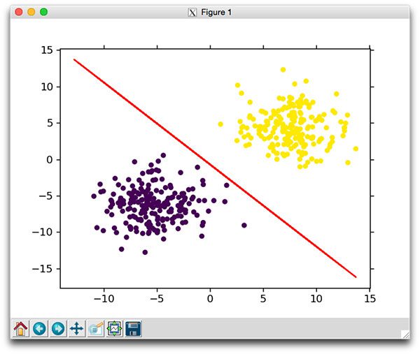
Figure 1: Learning the classification decision boundary using Stochastic Gradient Descent.
As the plot demonstrates, we are able to learn a weight matrix W that correctly classifies each of the data points.
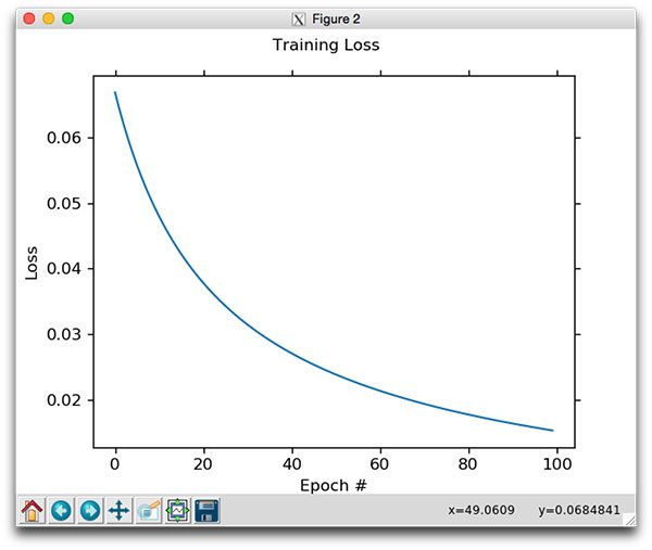
I have also included a plot that visualizes loss decreasing in further iterations of the Stochastic Gradient Descent algorithm:
Figure 2: The loss function associated with Stochastic Gradient Descent. Loss continues to decrease as we allow more epochs to pass.
Summary
In today’s blog post, we learned about Stochastic Gradient Descent (SGD), an extremely common extension to the vanilla gradient descent algorithm. In fact, in nearly all situations, you’ll see SGD used instead of the original gradient descent version.
SGD is also very common when training your own neural networks and deep learning classifiers. If you recall, a couple of weeks ago we used SGD to train a simple neural network. We also used SGD when training LeNet, a common Convolutional Neural Network.
Over the next couple of weeks I’ll be discussing some computer vision topics, but then we’ll pick up a thorough discussion of backpropagation along with the various types of layers in Convolutional Neural Networks come early November.
Be sure to use the form below to sign up for the PyImageSearch Newsletter to be notified when future blog posts are published!
Downloads:
The post Stochastic Gradient Descent (SGD) with Python appeared first on PyImageSearch.