A simple neural network with Python and Keras

Image Source

If you’ve been following along with this series of blog posts, then you already know what a huge fan I am of Keras.

Keras is a super powerful, easy to use Python library for building neural networks and deep learning networks.

In the remainder of this blog post, I’ll demonstrate how to build a simple neural network using Python and Keras, and then apply it to the task of image classification.

A simple neural network with Python and Keras

To start this post, we’ll quickly review the most common neural network architecture — feedforward networks.

We’ll then write some Python code to define our feedforward neural network and specifically apply it to the Kaggle Dogs vs. Cats classification challenge. The goal of this challenge is to correctly classify whether a given image contains a dog or a cat.

Finally, we’ll review the results of our simple neural network architecture and discuss methods to improve it.

Feedforward neural networks

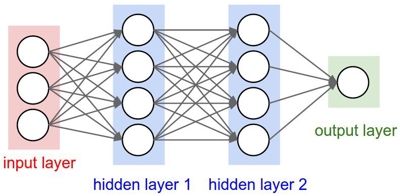
While there are many, many different neural network architectures, the most common architecture is the feedforward network:

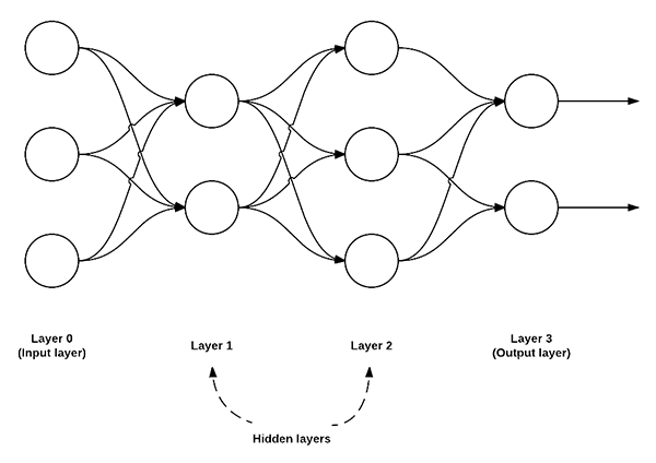
Figure 1: An example of a feedforward neural network with 3 input nodes, a hidden layer with 2 nodes, a second hidden layer with 3 nodes, and a final output layer with 2 nodes.

In this type of architecture, a connection between two nodes is only permitted from nodes in layer i to nodes in layer i + 1 (hence the term feedforward; there are no backwards or inter-layer connections allowed).

Furthermore, the nodes in layer i are fully connected to the nodes in layer i + 1. This implies that every node in layer i connects to every node in layer i + 1. For example, in the figure above, there are a total of 2 x 3 = 6 connections between layer 0 and layer 1 — this is where the term “fully connected” or “FC” for short, comes from.

We normally use a sequence of integers to quickly and concisely describe the number of nodes in each layer.

For example, the network above is a 3-2-3-2 feedforward neural network:

• Layer 0 contains 3 inputs, our values. These could be raw pixel intensities or entries from a feature vector.
• Layers 1 and 2 are hidden layers, containing 2 and 3 nodes, respectively.
• Layer 3 is the output layer or the visible layer — this is where we obtain the overall output classification from our network. The output layer normally has as many nodes as class labels; one node for each potential output. In our Kaggle Dogs vs. Cats example, we have two output nodes — one for “dog” and another for “cat”.

Implementing our own neural network with Python and Keras

Now that we understand the basics of feedforward neural networks, let’s implement one for image classification using Python and Keras.

To start, you’ll want to follow this tutorial to ensure you have Keras and the associated prerequisites installed on your system.

From there, open up a new file, name it

simple_neural_network.py

# import the necessary packages
from sklearn.preprocessing import LabelEncoder
from sklearn.cross_validation import train_test_split
from keras.models import Sequential
from keras.layers import Activation
from keras.optimizers import SGD
from keras.layers import Dense
from keras.utils import np_utils
from imutils import paths
import numpy as np
import argparse
import cv2
import os

We start off by importing our required Python packages. We’ll be using a number of scikit-learn implementations along with Keras layers and activation functions. If you do not already have your development environment configured for Keras, please see this blog post.

We’ll be also using imutils, my personal library of OpenCV convenience functions. If you do not already have

imutils

pip

$ pip install imutils

Next, let’s define a method to accept and image and describe it. In previous tutorials, we’ve extracted color histograms from images and used these distributions to characterize the contents of an image.

This time, let’s use the raw pixel intensities instead. To accomplish this, we define the

image_to_feature_vector

image

size

# import the necessary packages
from sklearn.preprocessing import LabelEncoder
from sklearn.cross_validation import train_test_split
from keras.models import Sequential
from keras.layers import Activation
from keras.optimizers import SGD
from keras.layers import Dense
from keras.utils import np_utils
from imutils import paths
import numpy as np
import argparse
import cv2
import os

def image_to_feature_vector(image, size=(32, 32)):
	# resize the image to a fixed size, then flatten the image into
	# a list of raw pixel intensities
	return cv2.resize(image, size).flatten()

We resize our

image

In this case, we resize our image to 32 x 32 pixels and then flatten the 32 x 32 x 3 image (where we have three channels, one for each Red, Green, and Blue channel, respectively) into a 3,072-d feature vector.

The next code block handles parsing our command line arguments and taking care of a few initializations:

# import the necessary packages
from sklearn.preprocessing import LabelEncoder
from sklearn.cross_validation import train_test_split
from keras.models import Sequential
from keras.layers import Activation
from keras.optimizers import SGD
from keras.layers import Dense
from keras.utils import np_utils
from imutils import paths
import numpy as np
import argparse
import cv2
import os

def image_to_feature_vector(image, size=(32, 32)):
	# resize the image to a fixed size, then flatten the image into
	# a list of raw pixel intensities
	return cv2.resize(image, size).flatten()

# construct the argument parse and parse the arguments
ap = argparse.ArgumentParser()
ap.add_argument("-d", "--dataset", required=True,
	help="path to input dataset")
args = vars(ap.parse_args())

# grab the list of images that we'll be describing
print("[INFO] describing images...")
imagePaths = list(paths.list_images(args["dataset"]))

# initialize the data matrix and labels list
data = []
labels = []

We only need a single switch here,

--dataset

Line 28 grabs the paths to our

--dataset

data

labels

Now that we have our

imagePaths

data

labels

# import the necessary packages
from sklearn.preprocessing import LabelEncoder
from sklearn.cross_validation import train_test_split
from keras.models import Sequential
from keras.layers import Activation
from keras.optimizers import SGD
from keras.layers import Dense
from keras.utils import np_utils
from imutils import paths
import numpy as np
import argparse
import cv2
import os

def image_to_feature_vector(image, size=(32, 32)):
	# resize the image to a fixed size, then flatten the image into
	# a list of raw pixel intensities
	return cv2.resize(image, size).flatten()

# construct the argument parse and parse the arguments
ap = argparse.ArgumentParser()
ap.add_argument("-d", "--dataset", required=True,
	help="path to input dataset")
args = vars(ap.parse_args())

# grab the list of images that we'll be describing
print("[INFO] describing images...")
imagePaths = list(paths.list_images(args["dataset"]))

# initialize the data matrix and labels list
data = []
labels = []

# loop over the input images
for (i, imagePath) in enumerate(imagePaths):
	# load the image and extract the class label (assuming that our
	# path as the format: /path/to/dataset/{class}.{image_num}.jpg
	image = cv2.imread(imagePath)
	label = imagePath.split(os.path.sep)[-1].split(".")[0]

	# construct a feature vector raw pixel intensities, then update
	# the data matrix and labels list
	features = image_to_feature_vector(image)
	data.append(features)
	labels.append(label)

	# show an update every 1,000 images
	if i > 0 and i % 1000 == 0:
		print("[INFO] processed {}/{}".format(i, len(imagePaths)))

The

data

# import the necessary packages
from sklearn.preprocessing import LabelEncoder
from sklearn.cross_validation import train_test_split
from keras.models import Sequential
from keras.layers import Activation
from keras.optimizers import SGD
from keras.layers import Dense
from keras.utils import np_utils
from imutils import paths
import numpy as np
import argparse
import cv2
import os

def image_to_feature_vector(image, size=(32, 32)):
	# resize the image to a fixed size, then flatten the image into
	# a list of raw pixel intensities
	return cv2.resize(image, size).flatten()

# construct the argument parse and parse the arguments
ap = argparse.ArgumentParser()
ap.add_argument("-d", "--dataset", required=True,
	help="path to input dataset")
args = vars(ap.parse_args())

# grab the list of images that we'll be describing
print("[INFO] describing images...")
imagePaths = list(paths.list_images(args["dataset"]))

# initialize the data matrix and labels list
data = []
labels = []

# loop over the input images
for (i, imagePath) in enumerate(imagePaths):
	# load the image and extract the class label (assuming that our
	# path as the format: /path/to/dataset/{class}.{image_num}.jpg
	image = cv2.imread(imagePath)
	label = imagePath.split(os.path.sep)[-1].split(".")[0]

	# construct a feature vector raw pixel intensities, then update
	# the data matrix and labels list
	features = image_to_feature_vector(image)
	data.append(features)
	labels.append(label)

	# show an update every 1,000 images
	if i > 0 and i % 1000 == 0:
		print("[INFO] processed {}/{}".format(i, len(imagePaths)))

# encode the labels, converting them from strings to integers
le = LabelEncoder()
labels = le.fit_transform(labels)

# scale the input image pixels to the range [0, 1], then transform
# the labels into vectors in the range [0, num_classes] -- this
# generates a vector for each label where the index of the label
# is set to `1` and all other entries to `0`
data = np.array(data) / 255.0
labels = np_utils.to_categorical(labels, 2)

# partition the data into training and testing splits, using 75%
# of the data for training and the remaining 25% for testing
print("[INFO] constructing training/testing split...")
(trainData, testData, trainLabels, testLabels) = train_test_split(
	data, labels, test_size=0.25, random_state=42)

Lines 59 and 60 handle scaling the input data to the range [0, 1], followed by converting the

labels

We then construct our training and testing splits on Lines 65 and 66, using 75% of the data for training and the remaining 25% for testing.

For a more detailed review of the data preprocessing stage, please see this blog post.

We are now ready to define our neural network using Keras:

# import the necessary packages
from sklearn.preprocessing import LabelEncoder
from sklearn.cross_validation import train_test_split
from keras.models import Sequential
from keras.layers import Activation
from keras.optimizers import SGD
from keras.layers import Dense
from keras.utils import np_utils
from imutils import paths
import numpy as np
import argparse
import cv2
import os

def image_to_feature_vector(image, size=(32, 32)):
	# resize the image to a fixed size, then flatten the image into
	# a list of raw pixel intensities
	return cv2.resize(image, size).flatten()

# construct the argument parse and parse the arguments
ap = argparse.ArgumentParser()
ap.add_argument("-d", "--dataset", required=True,
	help="path to input dataset")
args = vars(ap.parse_args())

# grab the list of images that we'll be describing
print("[INFO] describing images...")
imagePaths = list(paths.list_images(args["dataset"]))

# initialize the data matrix and labels list
data = []
labels = []

# loop over the input images
for (i, imagePath) in enumerate(imagePaths):
	# load the image and extract the class label (assuming that our
	# path as the format: /path/to/dataset/{class}.{image_num}.jpg
	image = cv2.imread(imagePath)
	label = imagePath.split(os.path.sep)[-1].split(".")[0]

	# construct a feature vector raw pixel intensities, then update
	# the data matrix and labels list
	features = image_to_feature_vector(image)
	data.append(features)
	labels.append(label)

	# show an update every 1,000 images
	if i > 0 and i % 1000 == 0:
		print("[INFO] processed {}/{}".format(i, len(imagePaths)))

# encode the labels, converting them from strings to integers
le = LabelEncoder()
labels = le.fit_transform(labels)

# scale the input image pixels to the range [0, 1], then transform
# the labels into vectors in the range [0, num_classes] -- this
# generates a vector for each label where the index of the label
# is set to `1` and all other entries to `0`
data = np.array(data) / 255.0
labels = np_utils.to_categorical(labels, 2)

# partition the data into training and testing splits, using 75%
# of the data for training and the remaining 25% for testing
print("[INFO] constructing training/testing split...")
(trainData, testData, trainLabels, testLabels) = train_test_split(
	data, labels, test_size=0.25, random_state=42)

# define the architecture of the network
model = Sequential()
model.add(Dense(768, input_dim=3072, init="uniform",
	activation="relu"))
model.add(Dense(384, init="uniform", activation="relu"))
model.add(Dense(2))
model.add(Activation("softmax"))

On Lines 69-74 we construct our neural network architecture — a 3072-768-384-2 feedforward neural network.

Our input layer has 3,072 nodes, one for each of the 32 x 32 x 3 = 3,072 raw pixel intensities in our flattened input images.

We then have two hidden layers, each with 768 and 384 nodes, respectively. These node counts were determined via a cross-validation and hyperparameter tuning experiment performed offline.

The output layer has 2 nodes — one for each of the “dog” and “cat” labels.

We then apply a

softmax

The next step is to train our model using Stochastic Gradient Descent (SGD):

# import the necessary packages
from sklearn.preprocessing import LabelEncoder
from sklearn.cross_validation import train_test_split
from keras.models import Sequential
from keras.layers import Activation
from keras.optimizers import SGD
from keras.layers import Dense
from keras.utils import np_utils
from imutils import paths
import numpy as np
import argparse
import cv2
import os

def image_to_feature_vector(image, size=(32, 32)):
	# resize the image to a fixed size, then flatten the image into
	# a list of raw pixel intensities
	return cv2.resize(image, size).flatten()

# construct the argument parse and parse the arguments
ap = argparse.ArgumentParser()
ap.add_argument("-d", "--dataset", required=True,
	help="path to input dataset")
args = vars(ap.parse_args())

# grab the list of images that we'll be describing
print("[INFO] describing images...")
imagePaths = list(paths.list_images(args["dataset"]))

# initialize the data matrix and labels list
data = []
labels = []

# loop over the input images
for (i, imagePath) in enumerate(imagePaths):
	# load the image and extract the class label (assuming that our
	# path as the format: /path/to/dataset/{class}.{image_num}.jpg
	image = cv2.imread(imagePath)
	label = imagePath.split(os.path.sep)[-1].split(".")[0]

	# construct a feature vector raw pixel intensities, then update
	# the data matrix and labels list
	features = image_to_feature_vector(image)
	data.append(features)
	labels.append(label)

	# show an update every 1,000 images
	if i > 0 and i % 1000 == 0:
		print("[INFO] processed {}/{}".format(i, len(imagePaths)))

# encode the labels, converting them from strings to integers
le = LabelEncoder()
labels = le.fit_transform(labels)

# scale the input image pixels to the range [0, 1], then transform
# the labels into vectors in the range [0, num_classes] -- this
# generates a vector for each label where the index of the label
# is set to `1` and all other entries to `0`
data = np.array(data) / 255.0
labels = np_utils.to_categorical(labels, 2)

# partition the data into training and testing splits, using 75%
# of the data for training and the remaining 25% for testing
print("[INFO] constructing training/testing split...")
(trainData, testData, trainLabels, testLabels) = train_test_split(
	data, labels, test_size=0.25, random_state=42)

# define the architecture of the network
model = Sequential()
model.add(Dense(768, input_dim=3072, init="uniform",
	activation="relu"))
model.add(Dense(384, init="uniform", activation="relu"))
model.add(Dense(2))
model.add(Activation("softmax"))

# train the model using SGD
print("[INFO] compiling model...")
sgd = SGD(lr=0.01)
model.compile(loss="binary_crossentropy", optimizer=sgd,
	metrics=["accuracy"])
model.fit(trainData, trainLabels, nb_epoch=50, batch_size=128,
	verbose=1)

To train our model, we’ll set the learning rate parameter of SGD to 0.01. We’ll use the

binary_crossentropy

In most cases, you’ll want to use just

crossentropy

binary_crossentropy

crossentropy

The network is then allowed to train for a total of 50 epochs, meaning that the model “sees” each individual training example 50 times in an attempt to learn an underlying pattern.

The final code block evaluates our Keras neural network on the testing data:

# import the necessary packages
from sklearn.preprocessing import LabelEncoder
from sklearn.cross_validation import train_test_split
from keras.models import Sequential
from keras.layers import Activation
from keras.optimizers import SGD
from keras.layers import Dense
from keras.utils import np_utils
from imutils import paths
import numpy as np
import argparse
import cv2
import os

def image_to_feature_vector(image, size=(32, 32)):
	# resize the image to a fixed size, then flatten the image into
	# a list of raw pixel intensities
	return cv2.resize(image, size).flatten()

# construct the argument parse and parse the arguments
ap = argparse.ArgumentParser()
ap.add_argument("-d", "--dataset", required=True,
	help="path to input dataset")
args = vars(ap.parse_args())

# grab the list of images that we'll be describing
print("[INFO] describing images...")
imagePaths = list(paths.list_images(args["dataset"]))

# initialize the data matrix and labels list
data = []
labels = []

# loop over the input images
for (i, imagePath) in enumerate(imagePaths):
	# load the image and extract the class label (assuming that our
	# path as the format: /path/to/dataset/{class}.{image_num}.jpg
	image = cv2.imread(imagePath)
	label = imagePath.split(os.path.sep)[-1].split(".")[0]

	# construct a feature vector raw pixel intensities, then update
	# the data matrix and labels list
	features = image_to_feature_vector(image)
	data.append(features)
	labels.append(label)

	# show an update every 1,000 images
	if i > 0 and i % 1000 == 0:
		print("[INFO] processed {}/{}".format(i, len(imagePaths)))

# encode the labels, converting them from strings to integers
le = LabelEncoder()
labels = le.fit_transform(labels)

# scale the input image pixels to the range [0, 1], then transform
# the labels into vectors in the range [0, num_classes] -- this
# generates a vector for each label where the index of the label
# is set to `1` and all other entries to `0`
data = np.array(data) / 255.0
labels = np_utils.to_categorical(labels, 2)

# partition the data into training and testing splits, using 75%
# of the data for training and the remaining 25% for testing
print("[INFO] constructing training/testing split...")
(trainData, testData, trainLabels, testLabels) = train_test_split(
	data, labels, test_size=0.25, random_state=42)

# define the architecture of the network
model = Sequential()
model.add(Dense(768, input_dim=3072, init="uniform",
	activation="relu"))
model.add(Dense(384, init="uniform", activation="relu"))
model.add(Dense(2))
model.add(Activation("softmax"))

# train the model using SGD
print("[INFO] compiling model...")
sgd = SGD(lr=0.01)
model.compile(loss="binary_crossentropy", optimizer=sgd,
	metrics=["accuracy"])
model.fit(trainData, trainLabels, nb_epoch=50, batch_size=128,
	verbose=1)

# show the accuracy on the testing set
print("[INFO] evaluating on testing set...")
(loss, accuracy) = model.evaluate(testData, testLabels,
	batch_size=128, verbose=1)
print("[INFO] loss={:.4f}, accuracy: {:.4f}%".format(loss,
	accuracy * 100))

Classifying images using neural networks with Python and Keras

To execute our

simple_neural_network.py

1. Downloaded the source code to this post by using the “Downloads” section at the bottom of this tutorial.
2. Downloaded the Kaggle Dogs vs. Cats dataset from the Kaggle competition page.

The following command can be used to train our neural network using Python and Keras:

$ python simple_neural_network.py --dataset kaggle_dogs_vs_cats

Note: You might need to rename your Kaggle dataset directory (or simply update the path supplied to

--dataset

The output of our script can be seen in the screenshot below:

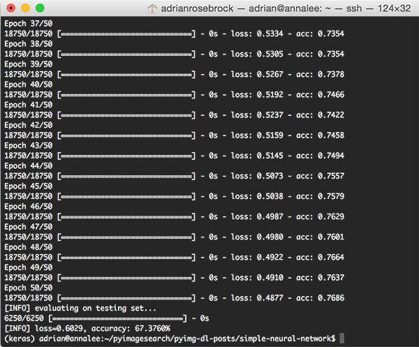
Figure 2: Training a simple neural network using the Keras deep learning library and the Python programming language.

On my Titan X GPU, the entire process of feature extraction, training the neural network, and evaluation took a total of 1m 15s with each epoch taking less than 0 seconds to complete.

At the end of the 50th epoch, we see that we are getting ~76% accuracy on the training data and 67% accuracy on the testing data.

This ~9% difference in accuracy implies that our network is overfitting a bit; however, it is very common to see ~10% gaps in training versus testing accuracy, especially if you have limited training data.

You should start to become very worried regarding overfitting when your training accuracy reaches 90%+ and your testing accuracy is substantially lower than that.

In either case, this 67.376% is the highest accuracy we’ve obtained thus far in this series of tutorials. As we’ll find out later on, we can easily obtain > 95% accuracy by utilizing Convolutional Neural Networks.

Summary

In today’s blog post, I demonstrated how to train a simple neural network using Python and Keras.

We then applied our neural network to the Kaggle Dogs vs. Cats dataset and obtained 67.376% accuracy utilizing only the raw pixel intensities of the images.

Starting next week, I’ll begin discussing optimization methods such as gradient descent and Stochastic Gradient Descent (SGD). I’ll also include a tutorial on backpropagation to help you understand the inner-workings of this important algorithm.

Before you go, be sure to enter your email address in the form below to be notified when future blog posts are published — you won’t want to miss them!

Downloads:

If you would like to download the code and images used in this post, please enter your email address in the form below. Not only will you get a .zip of the code, I’ll also send you a FREE 11-page Resource Guide on Computer Vision and Image Search Engines, including exclusive techniques that I don’t post on this blog! Sound good? If so, enter your email address and I’ll send you the code immediately!

Email address:

The post A simple neural network with Python and Keras appeared first on PyImageSearch.