Last week, we discussed Multi-class SVM loss; specifically, the hinge loss and squared hinge loss functions.
A loss function, in the context of Machine Learning and Deep Learning, allows us to quantify how “good” or “bad” a given classification function (also called a “scoring function”) is at correctly classifying data points in our dataset.
However, while hinge loss and squared hinge loss are commonly used when training Machine Learning/Deep Learning classifiers, there is another method more heavily used…
In fact, if you have done previous work in Deep Learning, you have likely heard of this function before — do the terms Softmax classifier and cross-entropy loss sound familiar?
I’ll go as far to say that if you do any work in Deep Learning (especially Convolutional Neural Networks) that you’ll run into the term “Softmax”: it’s the final layer at the end of the network that yields your actual probability scores for each class label.
To learn more about Softmax classifiers and the cross-entropy loss function, keep reading.
Looking for the source code to this post?
Jump right to the downloads section.
Softmax Classifiers Explained
While hinge loss is quite popular, you’re more likely to run into cross-entropy loss and Softmax classifiers in the context of Deep Learning and Convolutional Neural Networks.
Why is this?
Simply put:
Softmax classifiers give you probabilities for each class label while hinge loss gives you the margin.
It’s much easier for us as humans to interpret probabilities rather than margin scores (such as in hinge loss and squared hinge loss).
Furthermore, for datasets such as ImageNet, we often look at the rank-5 accuracy of Convolutional Neural Networks (where we check to see if the ground-truth label is in the top-5 predicted labels returned by a network for a given input image).
Seeing (1) if the true class label exists in the top-5 predictions and (2) the probability associated with the predicted label is a nice property.
Understanding Multinomial Logistic Regression and Softmax Classifiers
The Softmax classifier is a generalization of the binary form of Logistic Regression. Just like in hinge loss or squared hinge loss, our mapping function f is defined such that it takes an input set of data x and maps them to the output class labels via a simple (linear) dot product of the data x and weight matrix W:
 = Wx_{i}")
However, unlike hinge loss, we interpret these scores as unnormalized log probabilities for each class label — this amounts to swapping out our hinge loss function with cross-entropy loss:
")
So, how did I arrive here? Let’s break the function apart and take a look.
To start, our loss function should minimize the negative log likelihood of the correct class:
")
This probability statement can be interpreted as:
 = e^{s_{y_{i}}} / \sum_{j} e^{s_{j}}")
Where we use our standard scoring function form:
")
As a whole, this yields our final loss function for a single data point, just like above:
Note: Your logarithm here is actually base e (natural logarithm) since we are taking the inverse of the exponentiation over e earlier.
The actual exponentiation and normalization via the sum of exponents is our actual Softmax function. The negative log yields our actual cross-entropy loss.
Just as in hinge loss or squared hinge loss, computing the cross-entropy loss over an entire dataset is done by taking the average:

If these equations seem scary, don’t worry — I’ll be working an actual numerical example in the next section.
Note: I’m purposely leaving out the regularization term as to not bloat this tutorial or confuse readers. We’ll return to regularization and explain what it is, how to use, and why it’s important for machine learning/deep learning in a future blog post.
A worked Softmax example
To demonstrate cross-entropy loss in action, consider the following figure:
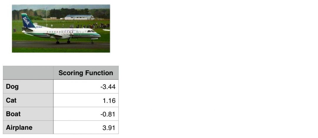
Figure 1: To compute our cross-entropy loss, let’s start with the output of our scoring function (the first column).
Our goal is to classify whether the image above contains a dog, cat, boat, or airplane.
Clearly we can see that this image is an “airplane”. But does our Softmax classifier?
To find out, I’ve included the output of our scoring function f for each of the four classes, respectively, in Figure 1 above. These values are our unnormalized log probabilities for the four classes.
Note: I used a random number generator to obtain these values for this particular example. These values are simply used to demonstrate how the calculations of the Softmax classifier/cross-entropy loss function are performed. In reality, these values would not be randomly generated — they would instead be the output of your scoring function f.
Let’s exponentiate the output of the scoring function, yielding our unnormalized probabilities:
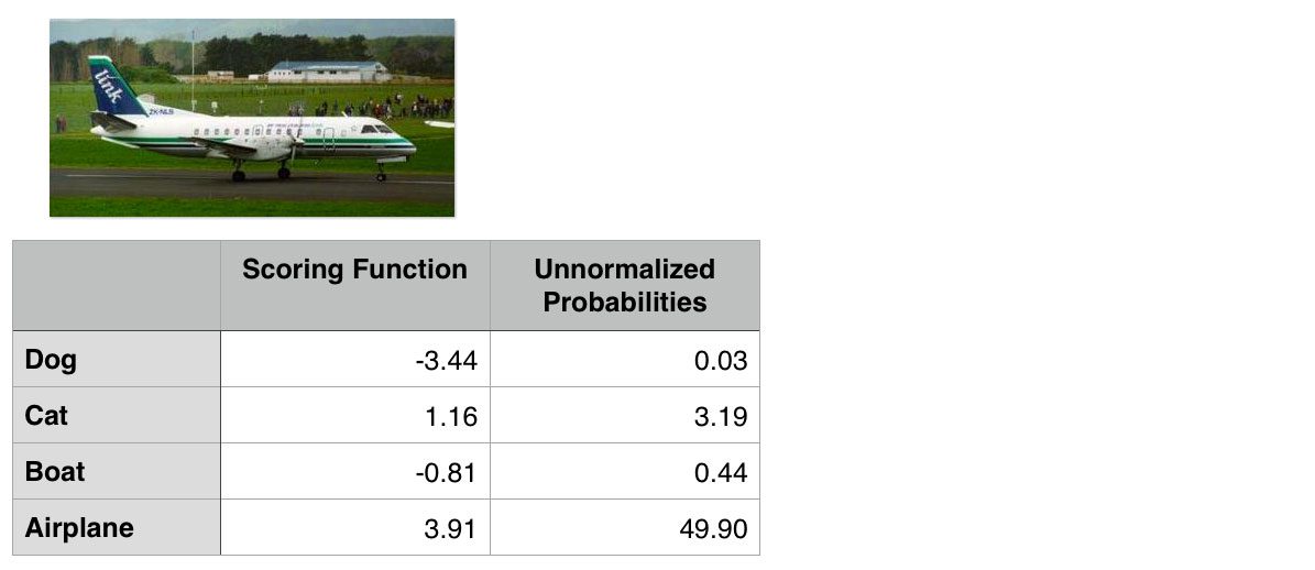
Figure 2: Exponentiating the output values from the scoring function gives us our unnormalized probabilities.
The next step is to take the denominator, sum the exponents, and divide by the sum, thereby yielding the actual probabilities associated with each class label:
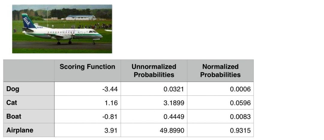
Figure 3: To obtain the actual probabilities, we divide each individual unnormalized probability by the sum of unnormalized probabilities.
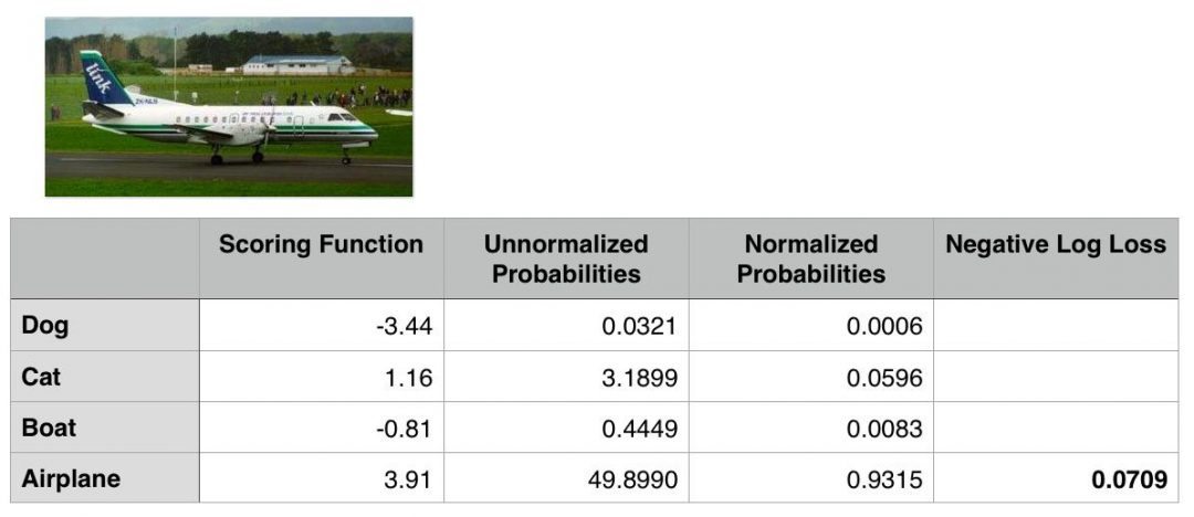
Finally, we can take the negative log, yielding our final loss:
Figure 4: Taking the negative log of the probability for the correct ground-truth class yields the final loss for the data point.
In this case, our Softmax classifier would correctly report the image as airplane with 93.15% confidence.
The Softmax Classifier in Python
In order to demonstrate some of the concepts we have learned thus far with actual Python code, we are going to use a SGDClassifier with a log loss function.
Note: We’ll learn more about Stochastic Gradient Descent and other optimization methods in future blog posts.
For this example, we’ll once again be using the Kaggle Dogs vs. Cats dataset, so before we get started, make sure you have:
- Downloaded the source code to this blog post used the “Downloads” form at the bottom of this tutorial.
- Downloaded the Kaggle Dogs vs. Cats dataset.
In our particular example, the Softmax classifier will actually reduce to a special case — when there are K=2 classes, the Softmax classifier reduces to simple Logistic Regression. If we have > 2 classes, then our classification problem would become Multinomial Logistic Regression, or more simply, a Softmax classifier.
With that said, open up a new file, name it
softmax.py, and insert the following code:
# import the necessary packages
from sklearn.preprocessing import LabelEncoder
from sklearn.linear_model import SGDClassifier
from sklearn.metrics import classification_report
from sklearn.cross_validation import train_test_split
from imutils import paths
import numpy as np
import argparse
import imutils
import cv2
import os
If you’ve been following along on the PyImageSearch blog over the past few weeks, then the code above likely looks fairly familiar — all we are doing here is importing our required Python packages.
We’ll be using the scikit-learn library, so if you don’t already have it installed, be sure to install it now:
$ pip install scikit-learn
We’ll also be using my imutils package, a series of convenience functions used to make performing common image processing operations an easier task. If you do not have
imutilsinstalled, you’ll want to install it as well:
$ pip install imutils
Next, we define our
extract_color_histogramfunction which is used to quantify the color distribution of our input
imageusing the supplied number of
bins:
# import the necessary packages
from sklearn.preprocessing import LabelEncoder
from sklearn.linear_model import SGDClassifier
from sklearn.metrics import classification_report
from sklearn.cross_validation import train_test_split
from imutils import paths
import numpy as np
import argparse
import imutils
import cv2
import os

def extract_color_histogram(image, bins=(8, 8, 8)):
	# extract a 3D color histogram from the HSV color space using
	# the supplied number of `bins` per channel
	hsv = cv2.cvtColor(image, cv2.COLOR_BGR2HSV)
	hist = cv2.calcHist([hsv], [0, 1, 2], None, bins,
		[0, 180, 0, 256, 0, 256])

	# handle normalizing the histogram if we are using OpenCV 2.4.X
	if imutils.is_cv2():
		hist = cv2.normalize(hist)

	# otherwise, perform "in place" normalization in OpenCV 3 (I
	# personally hate the way this is done
	else:
		cv2.normalize(hist, hist)

	# return the flattened histogram as the feature vector
	return hist.flatten()
I’ve already reviewed this function a few times before, so I’m going to skip the detailed review. For a more thorough discussion of
extract_color_histogram, why we are using it, and how it works, please see this blog post.
In the meantime, simply keep in mind that this function quantifies the contents of an image by constructing a histogram over the pixel intensities.
Let’s parse our command line arguments and grab the paths to our 25,000 Dogs vs. Cats images from disk:
# import the necessary packages
from sklearn.preprocessing import LabelEncoder
from sklearn.linear_model import SGDClassifier
from sklearn.metrics import classification_report
from sklearn.cross_validation import train_test_split
from imutils import paths
import numpy as np
import argparse
import imutils
import cv2
import os

def extract_color_histogram(image, bins=(8, 8, 8)):
	# extract a 3D color histogram from the HSV color space using
	# the supplied number of `bins` per channel
	hsv = cv2.cvtColor(image, cv2.COLOR_BGR2HSV)
	hist = cv2.calcHist([hsv], [0, 1, 2], None, bins,
		[0, 180, 0, 256, 0, 256])

	# handle normalizing the histogram if we are using OpenCV 2.4.X
	if imutils.is_cv2():
		hist = cv2.normalize(hist)

	# otherwise, perform "in place" normalization in OpenCV 3 (I
	# personally hate the way this is done
	else:
		cv2.normalize(hist, hist)

	# return the flattened histogram as the feature vector
	return hist.flatten()

# construct the argument parse and parse the arguments
ap = argparse.ArgumentParser()
ap.add_argument("-d", "--dataset", required=True,
	help="path to input dataset")
args = vars(ap.parse_args())

# grab the list of images that we'll be describing
print("[INFO] describing images...")
imagePaths = list(paths.list_images(args["dataset"]))

# initialize the data matrix and labels list
data = []
labels = []
We only need a single switch here,
--dataset, which is the path to our input Dogs vs. Cats images.
Once we have the paths to these images, we can loop over them individually and extract a color histogram for each image:
# import the necessary packages
from sklearn.preprocessing import LabelEncoder
from sklearn.linear_model import SGDClassifier
from sklearn.metrics import classification_report
from sklearn.cross_validation import train_test_split
from imutils import paths
import numpy as np
import argparse
import imutils
import cv2
import os

def extract_color_histogram(image, bins=(8, 8, 8)):
	# extract a 3D color histogram from the HSV color space using
	# the supplied number of `bins` per channel
	hsv = cv2.cvtColor(image, cv2.COLOR_BGR2HSV)
	hist = cv2.calcHist([hsv], [0, 1, 2], None, bins,
		[0, 180, 0, 256, 0, 256])

	# handle normalizing the histogram if we are using OpenCV 2.4.X
	if imutils.is_cv2():
		hist = cv2.normalize(hist)

	# otherwise, perform "in place" normalization in OpenCV 3 (I
	# personally hate the way this is done
	else:
		cv2.normalize(hist, hist)

	# return the flattened histogram as the feature vector
	return hist.flatten()

# construct the argument parse and parse the arguments
ap = argparse.ArgumentParser()
ap.add_argument("-d", "--dataset", required=True,
	help="path to input dataset")
args = vars(ap.parse_args())

# grab the list of images that we'll be describing
print("[INFO] describing images...")
imagePaths = list(paths.list_images(args["dataset"]))

# initialize the data matrix and labels list
data = []
labels = []

# loop over the input images
for (i, imagePath) in enumerate(imagePaths):
	# load the image and extract the class label (assuming that our
	# path as the format: /path/to/dataset/{class}.{image_num}.jpg
	image = cv2.imread(imagePath)
	label = imagePath.split(os.path.sep)[-1].split(".")[0]

	# extract a color histogram from the image, then update the
	# data matrix and labels list
	hist = extract_color_histogram(image)
	data.append(hist)
	labels.append(label)

	# show an update every 1,000 images
	if i > 0 and i % 1000 == 0:
		print("[INFO] processed {}/{}".format(i, len(imagePaths)))
Again, since I have already reviewed this boilerplate code multiple times on the PyImageSearch blog, I’ll refer you to this blog post for a more detailed discussion on the feature extraction process.
Our next step is to construct the training and testing split. We’ll use 75% of the data for training our classifier and the remaining 25% for testing and evaluating the model:
# import the necessary packages
from sklearn.preprocessing import LabelEncoder
from sklearn.linear_model import SGDClassifier
from sklearn.metrics import classification_report
from sklearn.cross_validation import train_test_split
from imutils import paths
import numpy as np
import argparse
import imutils
import cv2
import os

def extract_color_histogram(image, bins=(8, 8, 8)):
	# extract a 3D color histogram from the HSV color space using
	# the supplied number of `bins` per channel
	hsv = cv2.cvtColor(image, cv2.COLOR_BGR2HSV)
	hist = cv2.calcHist([hsv], [0, 1, 2], None, bins,
		[0, 180, 0, 256, 0, 256])

	# handle normalizing the histogram if we are using OpenCV 2.4.X
	if imutils.is_cv2():
		hist = cv2.normalize(hist)

	# otherwise, perform "in place" normalization in OpenCV 3 (I
	# personally hate the way this is done
	else:
		cv2.normalize(hist, hist)

	# return the flattened histogram as the feature vector
	return hist.flatten()

# construct the argument parse and parse the arguments
ap = argparse.ArgumentParser()
ap.add_argument("-d", "--dataset", required=True,
	help="path to input dataset")
args = vars(ap.parse_args())

# grab the list of images that we'll be describing
print("[INFO] describing images...")
imagePaths = list(paths.list_images(args["dataset"]))

# initialize the data matrix and labels list
data = []
labels = []

# loop over the input images
for (i, imagePath) in enumerate(imagePaths):
	# load the image and extract the class label (assuming that our
	# path as the format: /path/to/dataset/{class}.{image_num}.jpg
	image = cv2.imread(imagePath)
	label = imagePath.split(os.path.sep)[-1].split(".")[0]

	# extract a color histogram from the image, then update the
	# data matrix and labels list
	hist = extract_color_histogram(image)
	data.append(hist)
	labels.append(label)

	# show an update every 1,000 images
	if i > 0 and i % 1000 == 0:
		print("[INFO] processed {}/{}".format(i, len(imagePaths)))

# encode the labels, converting them from strings to integers
le = LabelEncoder()
labels = le.fit_transform(labels)

# partition the data into training and testing splits, using 75%
# of the data for training and the remaining 25% for testing
print("[INFO] constructing training/testing split...")
(trainData, testData, trainLabels, testLabels) = train_test_split(
	np.array(data), labels, test_size=0.25, random_state=42)

# train a Stochastic Gradient Descent classifier using a softmax
# loss function and 10 epochs
model = SGDClassifier(loss="log", random_state=967, n_iter=10)
model.fit(trainData, trainLabels)

# evaluate the classifier
print("[INFO] evaluating classifier...")
predictions = model.predict(testData)
print(classification_report(testLabels, predictions,
	target_names=le.classes_))
We also train our
SGDClassifierusing the
logloss function (Lines 75 and 76). Using the
logloss function ensures that we’ll obtain probability estimates for each class label at testing time.
Lines 79-82 then display a nicely formatted accuracy report for our classifier.
To examine some actual probabilities, let’s loop over a few randomly sampled training examples and examine the output probabilities returned by the classifier:
# import the necessary packages
from sklearn.preprocessing import LabelEncoder
from sklearn.linear_model import SGDClassifier
from sklearn.metrics import classification_report
from sklearn.cross_validation import train_test_split
from imutils import paths
import numpy as np
import argparse
import imutils
import cv2
import os

def extract_color_histogram(image, bins=(8, 8, 8)):
	# extract a 3D color histogram from the HSV color space using
	# the supplied number of `bins` per channel
	hsv = cv2.cvtColor(image, cv2.COLOR_BGR2HSV)
	hist = cv2.calcHist([hsv], [0, 1, 2], None, bins,
		[0, 180, 0, 256, 0, 256])

	# handle normalizing the histogram if we are using OpenCV 2.4.X
	if imutils.is_cv2():
		hist = cv2.normalize(hist)

	# otherwise, perform "in place" normalization in OpenCV 3 (I
	# personally hate the way this is done
	else:
		cv2.normalize(hist, hist)

	# return the flattened histogram as the feature vector
	return hist.flatten()

# construct the argument parse and parse the arguments
ap = argparse.ArgumentParser()
ap.add_argument("-d", "--dataset", required=True,
	help="path to input dataset")
args = vars(ap.parse_args())

# grab the list of images that we'll be describing
print("[INFO] describing images...")
imagePaths = list(paths.list_images(args["dataset"]))

# initialize the data matrix and labels list
data = []
labels = []

# loop over the input images
for (i, imagePath) in enumerate(imagePaths):
	# load the image and extract the class label (assuming that our
	# path as the format: /path/to/dataset/{class}.{image_num}.jpg
	image = cv2.imread(imagePath)
	label = imagePath.split(os.path.sep)[-1].split(".")[0]

	# extract a color histogram from the image, then update the
	# data matrix and labels list
	hist = extract_color_histogram(image)
	data.append(hist)
	labels.append(label)

	# show an update every 1,000 images
	if i > 0 and i % 1000 == 0:
		print("[INFO] processed {}/{}".format(i, len(imagePaths)))

# encode the labels, converting them from strings to integers
le = LabelEncoder()
labels = le.fit_transform(labels)

# partition the data into training and testing splits, using 75%
# of the data for training and the remaining 25% for testing
print("[INFO] constructing training/testing split...")
(trainData, testData, trainLabels, testLabels) = train_test_split(
	np.array(data), labels, test_size=0.25, random_state=42)

# train a Stochastic Gradient Descent classifier using a softmax
# loss function and 10 epochs
model = SGDClassifier(loss="log", random_state=967, n_iter=10)
model.fit(trainData, trainLabels)

# evaluate the classifier
print("[INFO] evaluating classifier...")
predictions = model.predict(testData)
print(classification_report(testLabels, predictions,
	target_names=le.classes_))

# to demonstrate that our classifier actually "learned" from
# our training data, randomly sample a few training images
idxs = np.random.choice(np.arange(0, len(trainData)), size=(5,))

# loop over the training indexes
for i in idxs:
	# predict class probabilities based on the extracted color
	# histogram
	hist = trainData[i].reshape(1, -1)
	(catProb, dogProb) = model.predict_proba(hist)[0]

	# show the predicted probabilities along with the actual
	# class label
	print("cat={:.1f}%, dog={:.1f}%, actual={}".format(catProb * 100,
		dogProb * 100, le.inverse_transform(trainLabels[i])))
Note: I’m randomly sampling from the training data rather than the testing data to demonstrate that there should be a noticeably large gap in between the probabilities for each class label. Whether or not each classification is correct is a a different story — but even if our prediction is wrong, we should still see some sort of gap that indicates that our classifier is actually learning from the data.
Line 93 handles computing the probabilities associated with the randomly sampled data point via the
.predict_probafunction.
The predicted probabilities for the cat and dog class are then displayed to our screen on Lines 97 and 98.
Softmax Classifier Results
Once you have:
- Downloaded both the source code to this blog using the “Downloads” form at the bottom of this tutorial.
- Downloaded the Kaggle Dogs vs. Cats dataset.
You can execute the following command to extract features from our dataset and train our classifier:
$ python softmax.py --dataset kaggle_dogs_vs_cats
After training our
SGDClassifier, you should see the following classification report:
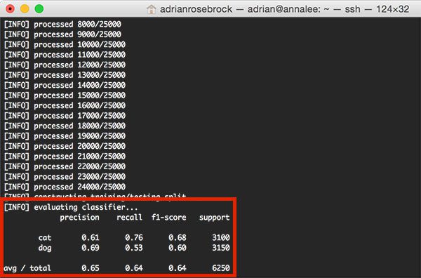
Figure 5: Computing the accuracy of our SGDClassifier with log loss — we obtain 65% classification accuracy.
Notice that our classifier has obtained 65% accuracy, an increase from the 64% accuracy when utilizing a Linear SVM in our linear classification post.
To investigate the individual class probabilities for a given data point, take a look at the rest of the
softmax.pyoutput:
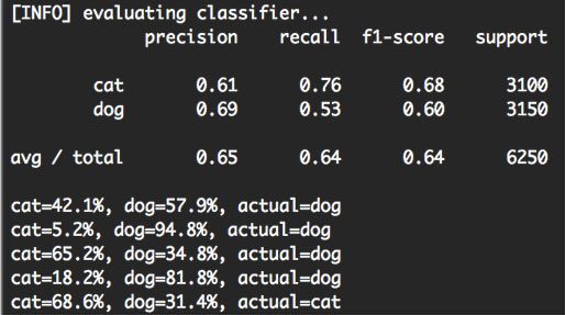
Figure 6: Investigating the class label probabilities for each prediction.
For each of the randomly sampled data points, we are given the class label probability for both “dog” and “cat”, along with the actual ground-truth label.
Based on this sample, we can see that we obtained 4 / 5 = 80% accuracy.
But more importantly, notice how there is a particularly large gap in between class label probabilities. If our Softmax classifier predicts “dog”, then the probability associated with “dog” will be high. And conversely, the class label probability associated with “cat” will be low.
Similarly, if our Softmax classifier predicts “cat”, then the probability associated with “cat” will be high, while the probability for “dog” will be “low”.
This behavior implies that there some actual confidence in our predictions and that our algorithm is actually learning from the dataset.
Exactly how the learning takes place involves updating our weight matrix W, which boils down to being an optimization problem. We’ll be reviewing how to perform gradient decent and other optimization algorithms in future blog posts.
Summary
In today’s blog post, we looked at the Softmax classifier, which is simply a generalization of the the binary Logistic Regression classifier.
When constructing Deep Learning and Convolutional Neural Network models, you’ll undoubtedly run in to the Softmax classifier and the cross-entropy loss function.
While both hinge loss and squared hinge loss are popular choices, I can almost guarantee with absolute certainly that you’ll see cross-entropy loss with more frequency — this is mainly due to the fact that the Softmax classifier outputs probabilities rather than margins. Probabilities are much easier for us as humans to interpret, so that is a particularly nice quality of Softmax classifiers.
Now that we understand the fundamentals of loss functions, we’re ready to tack on another term to our loss method — regularization.
The regularization term is appended to our loss function and is used to control how our weight matrix W “looks”. By controlling W and ensuring that it “looks” a certain way, we can actually increase classification accuracy.
After we discuss regularization, we can then move on to optimization — the process that actually takes the output of our scoring and loss functions and uses this output to tune our weight matrix W to actually “learn”.
Anyway, I hope you enjoyed this blog post!
Before you go, be sure to enter your email address in the form below to be notified when new blog posts go live!
Downloads:
The post Softmax Classifiers Explained appeared first on PyImageSearch.